1. Version Info

The latest version of RUBICS is v. 1.0.0 STAR. While the program is considered ‘feature complete’, it is still considered an early version of the software and it is not guaranteed that all of its functions have undergone extensive testing and verification. As such, users must exercise due caution when attempting to the use the program or interpret its outputs.

VERSION DATE: 09/06/2024

RUBICS is distributed under the GNU General Public License v3:

This program is free software: you can redistribute it and/or modify it under the terms of the GNU General Public License as published by the Free Software Foundation, either version 3 of the License, or (at your option) any later version.

This program is distributed in the hope that it will be useful, but WITHOUT ANY WARRANTY; without even the implied warranty of MERCHANTABILITY or FITNESS FOR A PARTICULAR PURPOSE. See the GNU General Public License for more details.

1.i. Source Code

RUBICS source code is maintained on GitHub

RUBICS is developed in Python v3.10.1 and utilises the following libraries:

• PySimpleGUI
• numpy
• scipy
• json
• datetime
• re
• pandas
• matplotlib
• World Bank API

No guarantees regarding the future functionality of RUBICS as a result of changes made to Python or any of the supporting libraries can be made.

2. User Settings

User settings are imported and exported in a .json file that is both human and machine readable to facilitate the saving and reviewing of previous CBAs.

The user settings file takes the form of a series of nested dictionaries that read to each of the major components as follows:

{
"monte_carlo_settings": {},
"discount_rate_settings": {},
"distribution_analysis_settings": {},
"reference_prices": {},
"event_model": {},
"quantity_scenarios": {}
}

monte_carlo_settings

The monte_carlo_settings sub-dictionary contains the values for setting the seed to be used in the random generators (for reproducibility) and the number of simulations to be run, for example:

{
"monte_carlo_settings": {
    "seed": 4328617,
    "n_simulations": 50000
    },
}

seed: integer

n_simulations: integer

probability distribution function settings

If any probability distribution functions are used in the analysis, the settings file will contain the function used and any of the parameters required, for example:

{
"discount_rate_settings": {
    "MC_PDF": "Uniform",
    "PDF_min": 0.7,
    "PDF_max": 1.35}
}

The following parameters are legal inputs into any PDF function from the settings file:

MC_PDF: string, any of: None, Uniform, Bounded normal-like, Triangular, PERT, Folded normal, Truncated normal, Exponential, Log-logistic, Log-normal, Custom Kinked PDF.

PDF_min: float

PDF_max: float

PDF_mean: float

PDF_stdev: float

PDF_mode: float

PDF_median: float

PDF_mode: float

PDF_shape: float

PDF_scale: float

PDF_lambda: float

PDF_Xs: list

PDF_Ys: list

discount_rate_settings

The discount_rate_settings sub-dictionary provides the information required to discounted future streams of costs and benefits. There are three different discount rate methods available, Constant, Stepped, and Gamma time declining. See section 4 for details on the discounting methods.

In addition, any Probability Distribution Function settings can be included with the discount rate settings. See section 3 for details on PDF functions.

– Constant discount rates

{
"discount_rate_settings": {
    "discounting_method": "Constant",
    "discount_rate": 7}
}

discounting_method: string

discount_rate: float

– Gamma time declining rates

{
"discount_rate_settings": {
    "discounting_method": "Gamma time declining",
    "discount_rate": 7,
    "discount_rate_sigma": 0.2}
}

discounting_method: string

discount_rate: float

discount_rate_sigma: float

– Stepped rates

{
"discount_rate_settings": {
    "discounting_method": "Stepped",
    "dr_step_range": ["0,5", "6,10", "11,20"],
    "dr_step_rates": [7, 5, 3],
    "dr_step_thereafter": 1}
}

discounting_method: string

dr_step_range: list of strings in format “start,end” period

dr_step_rates: list of floats

dr_step_thereafter: float

distribution_analysis_settings

Distribution analysis settings include one of two types: a simple_weight_matrix or an income weight matrix. See section Section 5 for information on their use and functions.

– simple_weight_matrix

{
"distribution_analysis_settings": {
    "simple_weight_matrix": [
        ["", "here", "there"],
        ["me", 1, 1],
        ["you", 1, 1],
        ["them", 1, 1],
    ]}
}

simple_weight_matrix: a table (list of lists) containing geographic zones in top row as strings, stakeholder groups in first column as strings, and weights in intersecting cells as float.

– income derived weights

{
"distribution_analysis_settings": {
    "population_average_income": 50,
    "income_weighting_parameter": 1.0,
    "subgroup_average_income": [
        ["", "here", "there"],
        ["me", 50, 60],
        ["you", 70, 80],
        ["them", 90, 100],
    ]}
}

population_average_income: float

income_weighting_parameter: float

subgroup_average_income: a table (list of lists) containing geographic zones in top row as strings, stakeholder groups in first column as strings, and incomes in intersecting cells as float.

Reference price settings

Reference price settings take a number of global variables followed by any number of nested price_group_n dictionaries. price_group_ dictionaries contain their own ID and PDF parameters, as well as any number of nested price_line_m dictionaries which contain the price data.

{
"reference_prices": {
    "country": "Australia",
    "year": 2023,
    "currency_conversion_range": "5 years",
    "currency_conversion_measure": "Median",

    "price_group_1": {
        "ID": "Group 1",
        "MC_PDF": "None",
        "price_line_1": {
            "ID": "Group 1 Line 1",
            "units": "Household",
            "nominal_value" 5.5,
            "currency": "AUS",
            "value_year": 2010,
            "adjustment_factor": 1.1,
            "MC_PDF": "None",
            "comments": "Source: Smith, A.(2011)"}
    }
}

country: string, any of countries listed in the ISO3 data sourced from the World Bank

year: integer, four digit

currency_conversion_range: string, any of 1 year, 2 years, 5 years, 10 years, 20 years, All dates.

currency_conversion_measure: string, any of Median, Mean

price_group_n: dictionary, where n in the number of the price group.

ID: string

price_line_m: dictionary, where m in the number of the price line.

units: string

nominal_value: float

currency: string, any abbreviated countries listed in the ISO3 data sourced from the World Bank

value_year: integer, four digit

adjustment_factor: float

comments: string

Event model settings

The event model settings takes the form of a series of nested dictionaries where event_e are the events and e is the event number, outcome_o are the outcomes where o is the outcome number, and scenario_s are the scenarios where s is the scenario number. Refer to section 7.iv for details on how inputs

{
"event_model": {
    "event_1": {
        "ID": "Natural Disaster",
        "event_depends": ""
        "outcome_1":{
            "ID": "Bushfire",
            "scenario_0": {
                "period_range": ["...", "0,10"],
                "outcome_weight: [1.0, 2],
                "periods_without_repeat: 2,
                "max_repeats": "None"},
            "scenario_1": {
                "period_range": ["<<<"],
                "outcome_weight: ["<<<"],
                "periods_without_repeat: "<<<",
                "max_repeats": "<<<"},
            },
        "outcome_2":{
            "ID": "No Bushfire",
            "scenario_0": {
                "period_range": ["...", "0,10"],
                "outcome_weight: [1.0, 1.5],
                "periods_without_repeat: 0,
                "max_repeats": "None"},
            "scenario_1": {
                "period_range": ["<<<"],
                "outcome_weight: ["<<<"],
                "periods_without_repeat: "<<<",
                "max_repeats": "<<<"},
            }
        }
    }
}

event_e: dictionary, where e is the event number.

ID: string

event_depends: string or list of strings, each string must refer to the ID of an outcome within another event.

outcome_o: dictionary, where o is the outcome number.

scenario_s: dictionary, where s is the scenario number.

period_range: list of strings, of format [start,end] periods or [“…”].

outcome_weight: list of floats or [“<<<“]

periods_without_repeat: integer or “<<<“

max_repeats: integer or “None” or “<<<“

Quantity Scenario settings

The quantity scenario settings takes the form of a series of nested dictionaries for each scenario_s where s is the scenario number, quantity_group_q where g is group number and quantity_line_u where u is the line number. Since the quantity scenarios section draws together all of the data provided in the reference prices, distribution analysis, and event model section, it is very important that those sections are complete and that the quantity scenarios settings do not reference fields or data that do not exist. Each scenario should ideally have the same number of groups and lines.

{
"quantity_scenarios": {
    "scenario_0": {
    "scenario_description": "Scenario without intervention",
    "quantity_group_1": {
        "ID": "Construction Costs",
        "group_value_type": "Costs",
        "MC_PDF": "None",

        "quantity_line_1": {
            "ID": "Building",
            "value": "Materials",
            "stakeholder_group": "Government",
            "geographic_zone": "State",
            "period_range": ["0,0"],
            "quantity": ["1.0"],
            "MC_PDF": "None",
            "outcome_dependency": "None",
            "comments": "Material Cost of Project"},
        "quantity_line_2": {
            "ID": "Community Benefits",
            "value": "WTP for Shelter",
            "stakeholder_group": "Households",
            "geographic_zone": "Regional State",
            "period_range": ["1,20"],
            "quantity": ["300"],
            "MC_PDF": "None",
            "outcome_dependency": "Bushfire",
            "comments": "Benefits occur in years when bushfires occur"}
        }
    }
}

scenario_s: dictionary where s is the number of the scenario.

scenario_description: string

quantity_group_q: dictionary where q is the number of the group.

ID: string

group_value_type: string, one of “Costs” or “Benefits”. All group value types across all scenarios are the same as in scenario 0.

quantity_line_u: dictionary, where u is the number of the line.

value: string, which is one of the IDs of the reference price lines in the CBA.

stakeholder_group: string, which is one of the stakeholder groups listed in the distribution analysis.

geographic_zone: string, which is one of the geographies listed in the distribution analysis.

period_range: list of string, of format [start:end] of each period.

quantity: list of floats or strings

outcome_dependency: string, which is one of the outcomes listed in the event model.

comments: string

2.i. Loading settings

When the user imports settings to RUBICS the program automatically generates any fields (such as price groups or lines) and overwrites any existing inputs for data that it reads in the file. However it does not delete existing data if there is no corresponding data in the settings file. Therefore, if a CBA is already loaded or populated, it is recommended that the analyst open a completely new instance of RUBICS before loading a new settings file unless they wish to compare the behaviour of two different variations of the same CBA.

2.i. Exporting settings

Exporting user settings functionality is currently not available (to be included in a future version). However, see section 8.ii. for a readout of the user settings formatted as a .json text file generated when the simulations are run.

2.iii. Ranges and rates

RUBICS requires the analyst to provide inputs to the UI in the form of period ranges and rates, for example:

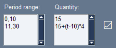
The input fields shown above allows the analyst to create functions over time (t) over different ranges. In the example, the analyst has defined two period ranges, the first from period 0 to period 10, and the second from period 11 to period 30. They have added two corresponding quantity functions, the first is a set rate of 15, and the second is an increasing function of time, adding 4 additional units per period. Clicking the graph symbol to the side brings up a useful popup that allows the analyst to check that their function is behaving as expected.

RUBICS reads the inputs naively from top to bottom, meaning that any overlapping ranges will overwrite previous ones. If the analyst writes 0,10 in the first line, and 7,20 in the second line, the function applying to line 1 will only be written over the periods 0,6.

There are two special shorthand inputs that apply to the event model builder only, since it would be exhausting to manually define event probabilities for each scenario when many of them are likely to be static and not different across scenarios. “…” in the period ranges input tells RUBICS that this period range is for all periods from 0 to the end of the analysis. “<<<” in the period ranges and rates inputs for scenarios 1 and up tells RUBICS that the ranges and rates are the same in this scenario as they are in scenario 0.

3. Probability Distribution Functions

RUBICS provides a number of probability distribution functions for use in various section of the CBA including the discount rates, reference prices, and quantity scenarios. These include:

• Uniform
• Bounded normal-like
• Triangular
• PERT
• Folded normal
• Truncated normal
• Exponential
• Log-logistic
• Log-normal
• Custom Kinked PDF

Outputs of the PDFs are designed to generate scale factors which are then multiplied by the variables (such as price or quantity) to generate random movement in the outcomes of the CBA. For example, if the analyst wished to consider a price with a most likely value of $5, with a variation +5% and -10%, then they might choose a triangular distribution of mode = 1, min=0.95, and max=1.10

In some cases, the mean of the PDF that the analyst has specified does not equal 1, which is what they might expect if their input is some reasonable central value for the variable. However, there are many cases where the base value, median, mode, and mean all differ significantly from one another and so RUBICS will only provide a warning to the analyst if this is the case.

– Uniform PDF

The uniform distribution is useful when the analyst has some idea regarding the range within which values are likely to fall, but no further information regarding the likely shape of the distribution.

RUBICS takes parameters min and max to generate random numbers from the uniform distribution. It uses the uniform.rvs() function from the scipy library to compute random numbers where loc=min and scale=(max-min).

– Bounded normal-like

The bounded normal-like function is described in Boardman et al. (2018) Cost-Benefit Analysis concepts and practice as a function that approximates a normal distribution within some bounded interval by taking the average of three uniformly distributed random numbers.

RUBICS takes parameters min and max to generate three random numbers from the uniform distribution (see above) and takes the mean to compute the final random number.

– Triangular

The triangular distribution is a useful distribution for when the analyst has some idea of the most likely value for a variable as well as a likely range. It can conveniently produce easily understandable asymmetrical distributions.

RUBICS takes parameters mode, min, and max to generate numbers from a triangular distribution. It uses the triang.rvs() function from the scipy library to compute random numbers where c=mode, loc=min, scale=(max-min).

– PERT

The PERT distribution offer a smoother function compared to the triangular distribution while also describing a distribution with some maximum likelihood values between a bounded range. It is commonly used in engineering application.

RUBICS takes parameters mode, min and max to generate random numbers from the PERT distribution. It uses the beta.rvs() function from the scipy library to compute random numbers using the formula:

min + beta.rvs(a, b, r)

Where:

a = 1 + 4 * (mode – min) / r

b = 1 + 4 * (max – mode) / r

r = max – min

– Folded normal

The folded normal distribution is provided to allow the analyst to use a normal distribution without having to worry about the possibility of producing negative factors which could lead to negative discount rates, prices or quantities, which are undesirable.

RUBICS takes parameters mean and sigma to generate random numbers from the folded normal distribution. It is important to note that the input parameters are the mean and sigma of the underlying normal distribution not the resulting distribution. It uses the foldnorm.rvs() function from the scipy library to compute random numbers where c=(mean/sigma), loc=0, and scale=sigma.

– Truncated normal

The truncated normal distribution is similar to the folded distribution and also provides a normal distribution to the analyst without the possibility of generating negative factors.

RUBICS takes parameters mean and sigma to generate numbers from the truncated normal distribution. It uses the truncnorm.rvs() function from the scipy library to compute random numbers where a=0, b=infinity, loc=mean, and scale=sigma.

– Exponential

The exponential function is useful for modelling many natural and social processes such as in hazard and survival analysis where events occur at some constant average rate. It has the useful property that the mean of the function is equal to 1/rate.

RUBICS takes the parameter rate to generate numbers from the exponential distribution. It uses the expon.rvs() function from the scipy library to compute random numbers where scale=1/rate.

– log-logistic

The log-logistic function produces a useful non-negative distribution which is useful for survival analysis as well as asymmetrical distributions of wealth. It has the useful property that that it can be defined from a median value.

RUBICS takes the parameters median and shape to generate numbers from the log-logistic function. It uses the fisk.rvs() function from the scipy library to compute random numbers where c=shape, and scale=median.

– log-normal

The log-normal distribution produces a useful non-negative distribution which has many applications in natural and social processes.

RUBICS takes the parameters mean and sigma to generate numbers from the log-normal function. It is important to note that this mean and sigma refer to the qualities of the underlying normal distribution function, not the qualities of the resulting log-normal function. The analyst should carefully study the behaviour of both before applying the function. It uses the lognorm.rvs() function from the scipy library to compute random numbers where s=sigma, and scale=exp(mean).

– custom kinked pdf

In some cases the analyst may wish to interpolate a continuous PDF from a set of X points with given Y weights.

RUBICS takes the set of X and Y points and uses the interp1d() function from the scipy library to create a custom function that is then subclassed by the rv_continuous class to create a PDF from which random variables may be drawn.

3.i. Correlated random variables

Under the Reference Prices section and the Quantity Scenarios section, variables can be assigned group-level random effects, and individual line-level random effects. This is because while some line item variables may be impacted by random variation, their variation may be correlated with other variables.

For example, while the cost of timber might vary between +/-15% and the cost of steel might vary +/-25% we might reasonably expect that the costs of all building materials will tend to increase or decrease together. In this case the analyst may choose to assign a group-level uniform PDF with a minimum of 0.9 and a maximum of 1.1. They would then assign an individual line item-level uniform PDF to timber (min=0.95, max=1.05) and a uniform PDF to steel (min=0.85, max=1.15).

Under this setup RUBICS computes a random group-level factor, and two individual-level factors. Say that the group level factor that is computed for a given simulation is 1.05, the factor computed for timber is 0.98, and the factor computed for steel is 1.11. The formula for random factor is given by:

overall random factor = group-level factor + individual-level factor – 1

Such that the overall random factor for timber is 1.05+0.98-1=1.03 and the overall random factor for steel is 1.05+1.11-1=1.16.

The analyst should carefully consider the variation they assign to the group-level and the individual line-level. Correlation of random variables will tend to increase the spread of the resulting CBA distribution, since non-correlated variables will tend to cancel each other out, they are therefore important to apply when necessary. However, care must be taken when mixing different PDFs to ensure that the analyst fully understands the beaviour of the system they are modelling.

4. Discount Rates

The practice of discounting future flows of costs and benefits is a fundamental part of CBA. However there is considerable variation in the rates that are applied in different jurisdictions and methods of doing so. RUBICS therefore offers three different methods, Constant, Stepped, and Gamma time declining.

The analyst is able to apply a Monte Carlo PDF over any of the discount rate methods. Doing so applies the random factor to the user input, that is, if the user input a discount rate of 7, and the random factor generate was 1.2, then the discount rate for the analysis in that simulation is 7*1.2=8.4. The rest of the discount rate procedure follows as usual.

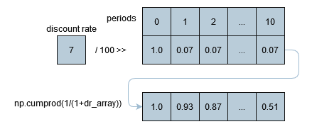
4.i. Constant discounting

The most common method of discounting applied, especially over short timescales, is a constant discount rate. For each period, RUBICS takes the constant discount rate provided and broadcasts it over an array of periods, before taking the cumulative product to arrive at the discount rate factor for each period except period 0, which is assumed to be the current period. For example, with a given input discount rate of 7%:

4.ii. Stepped discounting

Stepped discounting is a middle ground between the easily interpret-able nature of a constant discount rate and a time-declining discount rate favoured by many analysts for a variety of reasons. RUBICS uses the same method to compute stepped discounting factors for each period as the constant discounting procedure, with the exception that rates are applied over discrete periods specified by the analyst before a cumulative product is taken.

The analyst has the option of incorporating a discount rate as a function of time (see section 2.iii) if they wish to introduce their own continuous function over any range, although the analyst should of course take care to ensure that their function does not become negative over the domain of the analysis.

4.iii. Gamma time declining

Given that the entire premise of RUBICS is to examine how uncertainty impacts CBA it is interesting to consider the findings of Weitzman (2001) who note that the inherent uncertainty regarding the true discount rate leads to a expected value for the discount rate that declines over time.

Weitzman propose a formula for finding the discount rate at any period knowing the average value for the discount rate (mu) and its standard deviation (sigma):

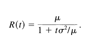
Applying this formula for the user-provided value for mu and sigma over the period array gives RUBICS the information needed to compute the discount rate factors for each period by a cumulative product as in section 4.i.

While RUBICS does not prevent the analyst from applying a Monte Carlo PDF over the Gamma time declining rate, they should carefully consider the extent to which doing so may be double counting the uncertainty in the analysis.

Weitzman, M. L. (2001). Gamma Discounting. American Economic Review, 91(1), 260–271. https://doi.org/10.1257/aer.91.1.260

5. Distribution Analysis

The RUBICS distribution analysis requires impacted groups to be defined by both a stakeholder group tag (such as ‘households’, ‘businesses’, ‘women’) and a geographic zone tag (such as ‘within state’, ‘cityburg’, ‘upriver’). Combined with the consideration of time inherent in CBA analysis, it is considered that this gives a nearly complete space-time-society view of the analysis. In addition, it is often a point of contention when a certain group (usually delineated by an arbitrary geographic boundary) lacks standing a CBA even if they are impacted by considerable costs/benefits. By providing an explicit place to account for these cases, RUBICS seeks to make it easier for the analyst to simultaneously report on in- and out-of-scope impacts without tedious re-analysis.

It is a deliberate design choice that RUBICS automatically computes a unit distribution weight matrix if no other weighting strategy is provided by the analyst. The reason for this is that unit weights are often implied by most CBAs as the default approach, rather than being reported as a deliberate assumption. However it is not clear that a unit weight approach is necessarily always the best economic strategy, given that it can enforce a ‘one-dollar one-vote’ rule rather than the more equitable ‘one-person one-vote’ rule. Therefore, since RUBICS seeks to encourage transparency, it is considered best to always show a weight matrix.

5.i. Basic weight matrix

If the analyst chooses to input basic weights calculated using their own methodology, such as a multi-criteria analysis survey or literature review, then they can apply any weights that they choose to the weight matrix.

Weights are simply multiplied by the final values computed by the CBA when the results are generated.

5.ii Income weight matrix

Based on the theory of social welfare functions, implying a declining marginal utility of income, a defined relationship between utility and income can be used to generate weights for use in CBA. Nurmi and Ahtiainen (2018) provide a detailed summary of the literature and economic theory, and provide the mathematical foundation for RUBICS to generate income derived weights.

The weight for a specific sub-group with average income y, given the population average income Y, and an income weighting parameter sigma is given by:

w = (y/Y)^(sigma)

Note that an income weighting parameter of 0 implies no income weighting. A value of 1.0 implies an income-weighted approach where one person equals one vote. A value greater than 1.0 implies a concave social welfare function where incremental improvements in monetary welfare are worth more to people with lower incomes than higher ones. Nurmi and Ahtiainen report a wide range of estimates. However, it is the goal of RUBICS to enable the analyst to easily review the consequences of their assumptions on any given set of results.

Nurmi, V., & Ahtiainen, H. (2018). Distributional Weights in Environmental Valuation and Cost-benefit Analysis: Theory and Practice. Ecological Economics, 150, 217–228. https://doi.org/10.1016/j.ecolecon.2018.04.021

6. Reference Prices

Reference prices must often be adjusted by various factors before they can be used in a CBA. RUBICS attempts to automate as much of the conversion processes as possible by accounting for CPI and Exchange Rates, and providing options for the user to alter how they are computed.

RUBICS uses data sourced from the World Bank API python library to obtain global datasets of CPI (1987-latest year available) and exchange rates (1960-latest year available). It is possible to update the World Bank data, however, this is conditional on the functionality of the API, which is not guaranteed.

After CPI and Currency Conversions are accounted for, the analyst has the option of incorporating another adjustment factor, such as one that converts a per household value to a per person metric, or any other reason. The real adjusted value used in the CBA is simply the nominal value multiplied by the currency conversion, the CPI factor, and the user-provided adjustment factor.

6.i. CPI conversions

RUBICS uses data sourced from the World Bank API python library to obtain CPI data for the purposes of obtaining prices in current values. For verification, the command to access the data in python, using pandas, is:

wb.data.DataFrame('FP.CPI.TOTL', time=range(1960, current_year+1), db=2)

RUBICS computes the real value by taking the CPI factor for the most recent year available (which may not necessarily be the current year), and dividing it by the CPI factor for the year provided in the price line.

6.ii. Exchange rate conversions

RUBICS uses data sourced from the World Bank API python library to obtain exchange rate data in national units of currency per USD. For verification, the command to access the data in python, using pandas, is:

wb.data.DataFrame('DPANUSSPB', time=range(1987, current_year+1), db=15)

Because exchange rates can fluctuate in a way that makes consistent analysis sometimes difficult on a year-on-year basis, the analyst has the option of specifying whether to take the median or mean exchange rate for the two currencies over a given period of time. For example, if the analyst selects a 5 year window and a median value, RUBICS will search the World Banks database for the most recent 5 year period of data available and return the median rate.

Converting between the two currencies is simply the value of the home currency in USD divided by the value of the foreign currency in USD for the same window of time and metric.

7. Quantity Scenarios

The quantity scenarios page is where action happens in RUBICS, here the analyst combines reference prices, stakeholders, probabilistic event outcomes, and quantities to define several scenarios representing alternative future states.

7.i. Scenarios

Because RUBICS assumes that the analyst will always wish to compare at least two scenarios, usually a state without intervention and a state (or more) with intervention, it automatically loads a scenario 0 and 1 upon opening. Of course, for simple analyses, the analyst is free to use only one.

However, the analyst should keep in mind that scenario 0 is a special case for a number of reasons. Group type (Costs or Benefits) can only be set in scenario 0, and are copied across to all the other scenarios from there. This is to ensure that each scenario can be compared to each other on an apples to apples (or rather, line by line) basis. In addition, when results are generated, the analyst has the opportunity to view scenarios 1+ net of scenario 0 in order to obtain the incremental net benefit, if required.

A note with regards to the generation of random effects via the probability distribution functions: random effects are separately and independently generated for each scenario. For example, if one defines a uniform PDF +/-10% for a given Quantity Group/Line for both scenario 0 and 1, then in an individual simulation the random effect generator may nudge scenario 0 up by 5% and scenario 1 down -3% even if they are intended to be identical. Therefore, it is important not to consider any individual simulation, rather, the entire distribution of the results should be taken into account where we expect these inconsistencies to wash out after thousands of simulations. If the analyst requires that random variables are generated only once – then they should take advantage of the Parameters. RUBICS was deliberately designed to allow random effects to be independently generated within each scenario for quantities, since some interventions that the analyst may wish to investigate could include, for example, lowering the probable consequence associated with a negative event, such as in climate risk mitigation, where a separate PDF for that line item in that scenario can be defined.

7.ii. Quantity groups

Quantity groups serve to organise CBA line items into digestible categories. The analyst should have at least two groups in a CBA, one for Costs and another for Benefits, however, they may include as many sub-categories as they require. For example, a CBA may contain a group for Construction Costs, Operation Costs, Community Benefits, Environmental Benefits, etc.

7.iii. Quantity lines

The analyst is required to fill several fields properly in order to complete a valid quantity line. Unlike the Group Type, nearly all the information

The Value dropdown list contains a list of all the values currently in the reference price section. RUBICS will display the real adjusted value and the units to assist the analyst in correctly identifying the relevant quantities. If the Value used is different between scenarios, it implies that the cost per unit under those scenarios is different.

The Stakeholder Group and Geographic Zone dropdown lists contain all the stakeholders and zones identified in the Distribution Analysis Settings. These are not mandatory since RUBICS can compute the CBA without any distributional information. However, if the analyst is using distribution groups, it is recommended that the analyst fill the Stakeholder Group and Geographic Zone inputs for all lines. If the stakeholder or zone identified in the lines are different between scenarios, it implies that there is a transfer between groups where a cost/benefit that accrues to one group in one scenario accrues instead to another in a different scenario.

The Period Range and Quantity fields allow the analyst to define the quantities of units over discrete time periods. See section 2.iii. for additional information on defining these ranges.

The Event Outcome Dependency requires the analyst to select which, of any, outcomes need to occur in any given time period in order for the quantities to be counted in the simulation. Here, the analyst can only select one available outcome from the Event Model, however if the analyst wishes to make the line dependent on multiple outcomes, they can instead make the outcome itself dependent on multiple other outcomes within the Event Model.

7.iv. Event Model

The Event Model Builder is a separate popup that enables the analyst to define chains of probabilistic Event-Outcomes that impact whether certain Quantity Lines in the CBA occur in any given time period.

The easiest way to begin designing an Event Model is to start with a tree diagram. For example, consider the case where we are interested in the consequences of a flood impacting a popular holiday town. If there is a 50% chance of a flood occurring or not occurring, we can weight these first outcomes equally. If a flood occurs, we should consider whether or not school holidays are on by making the School Holidays event dependent on the outcome of a flood occurring. Of course, the incidence of school holidays is completely independent of whether or not a flood occurs, but since we are not interested in whether school holidays are on when a flood does not occur, we can simplify the Event Model. In this case, there is a 10% chance that school holidays are on at the same time as flood occurs. We can then define two Disaster Level Events, each leading to a single outcome, Extreme and Dangerous respectively.

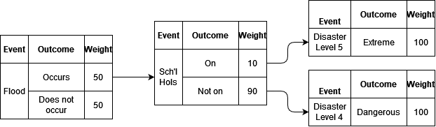
The analyst is free to alter the weights over time and across different scenarios. For example, climate change might mean that floods are more likely to occur in future periods, or an proposed intervention such as a levy in a particular scenario lowers the probability of the town flooding, or perhaps in another scenario the government deems school holidays too risky and decides to keep schools open during December and January.

Two additional input fields are provided to allow greater control of the rate of incidence of outcomes. The first is Periods Without Repetition, if this field is set to a value greater than 0, RUBICS will set the weight of that outcome to 0 for that number of time periods in the future if it occurs during any given simulation. The second is Maximum Number of Repetitions, if this field is set to anything other than ‘None’, if the event occurs within a given time period within a simulation, RUBICS will sum the number of total number of occurrences, and if this meets or exceeds the number of maximum repetitions, it will set all future weights for that outcome to 0.

It is important to note that the random generation of events is run once for each simulation and applied to each scenario since the Event Modeller uses a simple uniform random number generator between 0,1 to select which outcome should occur. This way if an outcome has a 0.50 chance of occurring in scenario 0 and a 0.70 chance of occurring in scenario 1, if the Monte Carlo simulation generates a roll of 0.60 in that time period, then the outcome will occur in scenario 0 but will not occur in scenario 1. This way it is possible to see how changes in risk affect outcomes.

8. Custom Parameters

Parameters are similar to Reference Prices and Quantities in that they are defined as a specific value over a specific time period. They can also be radomised using a probability distribution function.

However, they are also special, since parameters themselves can be used as inputs into Reference Prices, Quantities, or even other parameters. This makes them extraordinarily powerful for considering the impact of joint probabilities. In the example below a parameter ‘capcost’ is defined as a random variable, and is also used as an input into another parameter called ‘om’, which is itself also random.

"parameter_1": {
      "ID": "capcost",
      "period_range": [
        "0,34"
      ],
      "value": [
        "1608"
      ],
      "MC_PDF": "PERT",
      "PDF_min": 1.0,
      "PDF_mode": 1.49,
      "PDF_max": 9.25,
      "PDF_rand_each_t": false,
      "comments": "EIS Table 4.9. Noting that $1.61 billion relates to P50 costs, discounted over several years. Includes design and construction, project management, insurance, environmental controls, stakeholder engagement, legal and regulatory requirements, and contingency allowances. Does not include any environmental offset costs. Uncertainty intervals parametised from Petheram, C., & McMahon, T. A. (2019). Dams, dam costs and damnable cost overruns. Journal of Hydrology X, 3, 100026. https://doi.org/10.1016/j.hydroa.2019.100026."
    },
    "parameter_2": {
      "ID": "om",
      "period_range": [
        "0,34"
      ],
      "value": [
        "capcost*0.0021"
      ],
      "MC_PDF": "Triangular",
      "PDF_min": 0.38,
      "PDF_max": 4.10,
      "PDF_mode": 1.0,
      "PDF_rand_each_t": false,
      "comments": "Uncertainty interval parametised from Petheram, C., & McMahon, T. A. (2019). Dams, dam costs and damnable cost overruns. Journal of Hydrology X, 3, 100026. https://doi.org/10.1016/j.hydroa.2019.100026."
    }

The ‘capcost’ parameter is then used later in the Reference Prices as an input into a specific line item, as shown below:

"price_line_1": {
        "ID": "Construction",
        "units": "Annual",
        "nominal_value": "capcost",
        "currency": "AUS",
        "value_year": 2023,
        "adjustment_factor": 1.28,
        "MC_PDF": "None",
        "comments": "Updated to 2023 values by Other heavy and civil engineering construction PPI."
      }

9. Custom functions

While it is perfectly possible to prameterise an explicit function using nested parameters, as shown above, it is occasionally useful to be able to define a function from a set of x and y data points if they are somewhat noisy, or do not neatly fit into a neat family of parametric families. This is especially the case where one has frequency data, and has converted that into a piecewise cumulative distribution function, and would like to sample it without having to undergo the cumbersome task of integrating a probability distribution function from it. This is even more useful when such PDFs are expected to change over time, so that what one wants is some weighted average between the two.

Before an analyst uses an interpolation method to generate a custom function from an array of x and y values, they should consult the scipy documentation to ensure that they understand the procedure being undertaken. When in doubt, the analyst should always resort to defining a linear function from noisy data, for example using regression analysis, or simplifying the data so that a linear interpolation method can be reasonably applied.

The following interpolation methods are available for creating non-linear functions from an array of x and y points:

• Nearest – interpolate.interp1d(xs, ys, kind=’nearest’)
• Previous – interpolate.interp1d(xs, ys, kind=’previous’)
• Next – interpolate.interp1d(xs, ys, kind=’next’)
• Linear – interpolate.interp1d(xs, ys, kind=’linear’)
• Cubic Spline – interpolate.CubicSpline(xs, ys)
• Akima – interpolate.Akima1DInterpolator(xs, ys)
• Smoothed cubic spline – interpolate.UnivariateSpline(xs, ys, s=(smoother*max_sq_resids))
  where:
  smoother = a value provided by the user
  max_sq_resids = interpolate.UnivariateSpline(xs, ys, s=np.inf).get_residual()
  
  The user may note that the maximum practical value for s is the number of squared residuals when the number of knots equals 2. Since the UnivariateSpline starts at 2 knots and increases them until the squared residuals are lower than a given s, setting s to np.inf forces the knots to equal 2, and the maximum allowable s value can be determined. From there, a normalised smoother variable can be used to determined a practically useful value for s.

For example, the code block below shows two functions that outline a Point Probability Function (an inverted CDF) at the start of an analysis period ‘FhhBC’, and another for the end of the analysis period ‘FhhBCend’.

"function_1": {
      "ID": "FhhBC",
      "interpolation_method": "Linear",
      "x_values": [0, 0.5, 0.75, 0.9, 0.95, 0.975, 0.99, 0.995, 0.998, 0.999, 1.0],
      "y_values": [730, 1670, 2500, 4800, 7600, 10000, 15500, 19600, 23600, 26200, 36700],
      "comments": "Total number of houses impacted in the base case as a function of the flood severity. At year 2018"
    },
    "function_2": {
      "ID": "FhhBCend",
      "interpolation_method": "Linear",
      "x_values": [0, 0.5, 0.75, 0.9, 0.95, 0.975, 0.99, 0.995, 0.998, 0.999, 1.0],
      "y_values": [730, 1670, 2500, 4800, 7600, 10313, 18125, 25625, 34375, 39375, 60000],
      "comments": "Total number of houses impacted in the base case as a function of the flood severity. At year 2040"
    }

In the Parameters section, a random uniform variable ‘fld’ between 1 and 0 is created, which is then used to sample the PPFs defined above to generate the number of houses impacted in a given flood if it has occured at the beginning or end of the analysis period – the weighted average of which at each specific time step is then used to inform the analysis of how many houses are impacted in each year.

"parameter_3": {
      "ID": "fld",
      "period_range": [
        "0,34"
      ],
      "value": [
        "1"
      ],
      "MC_PDF": "Uniform",
      "PDF_min": 0,
      "PDF_max": 1,
      "PDF_rand_each_t": true,
      "comments": "Randomly generated probability points for flood severity percentile."
    },
    "parameter_4": {
      "ID": "hhBC",
      "period_range": [
        "0,17",
        "18,34"
      ],
      "value": [
        "(FhhBC(fld)*(23-(t+6))+FhhBCend(fld)*(t+6))/23",
        "FhhBCend(fld)"
      ],
      "MC_PDF": "None",
      "comments": "Number of houses impacted in the base case. Taking the weighted average of houses impacted in 2018 to 2040."
    }

10. Results

10.i. Initialisation

RUBICS requires a seed to be set for the purposes of ensuring reproducibility and uses the numpy random.default_rng() to set the global seed for all random number generators. In order to encourage analysts to avoid common seeds such as 0, 100, or 12345, RUBICS automatically populates the seed input with the milliseconds on the clock at the time of opening the program, which is about as random as you can get without knowing exactly how fast your computer is and having very quick reflexes.

The only other input required is the number of simulation to run. RUBICS automatically suggests 50,000, although the actual number needed to achieve a stable result will naturally vary between CBAs of greater or lower complexity. As a rule, the analyst should increment upwards the number of simulations until the results converge to a stable value across the entire distribution.

10.ii. Outputs

After clicking Run Monte Carlo Analysis, RUBICS executes the following steps to produce the summary results:

1. Set seed and random_generator from the seed value provided.
2. Set the number of simulation (S) from the value provided.
3. Search all of the Period Ranges supplied in the Quantity Scenarios Tab for the maximum to set the number of periods (T) required for each simulation (s).
4. Calculate the discount rates for each period (t) as a 1xT array.
5. Generate S random numbers from the Discount Rate PDF settings required as an Sx1 array.
6. Calculate the discount rate factors for all t and s by taking the cumulative product along the row axis of 1 – the matrix multiplication of e4. and e5.
7. Generate S random numbers for the Price Group PDF settings required as separate arrays.
8. Generate S random numbers for the Price Line PDF settings required as separate arrays.
9. Calculate prices for each Price Line as real_adjusted_value*(e7. + e8. – 1)
10. In order of Events without outcome dependencies to those that do, generate an SxT array of uniformly distributed random numbers between 0 and 1.
11. Stack all binary arrays that the Event is depended on calculated in previous iteration. Multiply by an SxT unit array to create the event dependency mask.
12. Generate an 1xT array of weights for each outcome of the event. Stack each array to produce an OxT aray where O is the number of outcomes.
13. For each s in each t, divide each outcome (o) in e12. by the sum of weights in t and take the cumulative sum.
14. Minus 10.[s, t] from each o and find the index of the lowest non-zero number to find the outcome that has occurred in that t.
15. Check if the the outcome that has occurred has any periods without repetition. If yes, set all weights for that outcome in e12. for that many periods in the future to zero.
16. Check if the outcome that has occurred has exceeded it maximum number of repeats. If yes, set all weights for that outcome in e12. for all future periods to zero.
17. Create an SxT boolean array for each outcome where True = occurred.
18. For each scenario, generate a 1xT array of quantities.
19. For each scenario, generate Sx1 random numbers from the Quantity Group PDF settings as required.
20. For each scenario, generate Sx1 random numbers from the Quantity Line PDF settings as required.
21. Calculate quantities for each Quantity Line as e18 x (e19. + e20. – 1).
22. Mask the quantity streams from e20. where the outcome dependencies calculated from e17 are False.
23. Multiply e22. by e9. to obtain SxT nominal prices for each quantity line.
24. Multiply e23. by e6. to obtain SxT present values for each quantity line.
25. Sum over s24 to obtain Sx1 total present value for each quantity line.
26. Take summary statistics of s25. (mean and percentiles using np.percentile(method=’linear’))

– CBA readout

After the procedure outlined above has been executed, RUBICS aggregates the data by scenario, type (costs and benefits), group, and line and displays it in a readout that can be copy-pasted into any word processor or workbook. The analyst has several further options to refine and review the outcomes of the CBA.

If Scenarios 1+ net of Scenario 0 is set to ‘Yes’ then all of the scenarios will take the difference of Scenario 0.

Monte Carlo Results to Display selects the Average or the Percentile to show in the CBA RESULTS readout.

If a Distribution Analysis has been used in the CBA, the analyst can check or uncheck the radio boxes provided to filter the results.

The BCR denominator dropdown allows the analyst to select which cost group should appear in the denominator (with all other costs appearing as negative values in the numerator). This is intended to allow the analyst to calculate, for example, the net benefits per unit of of capital investment or other ‘constrained’ costs. While Boardman et al (2018) correctly identify that arbitrary manipulation of the BCR can lead to misleading results, deliberately formulated variations of the BCR are often used for specific purposes; see ESCCH (2021) and Pannell (2019) for an in-depth discussion.

Earth Systems and Climate Change Hub. (2021). The Australian guide to nature-based methods for reducing risk from coastal hazards (No. 26). https://nespclimate.com.au/wp-content/uploads/2021/05/Nature-Based-Methods_Final_05052021.pdf

Pannell, D. (2019). 324. NPV versus BCR part 3 – Pannell Discussions. https://www.pannelldiscussions.net/2019/09/324-npv-vs-bcr-3/